Tutorial: Rectangular Waveguide
From openEMS
- Download the latest matlab file using Github: Rect_Waveguide.m
- Simulation Time: ~ 5 min for a 5m long waveguide
We will cover in this tutorial:
- setup a mode profile excitation,
- create voltage and current probes using the mode profile,
- calculate and plot the waveguide impedance and s-parameters.
Octave (Matlab) Simulation Script
To start the script within an empty environment, the first lines are:
close all
clear
clc
Setup the simulation, starting with the units:
physical_constants;
unit = 1e-6; %drawing unit in microns
Next, specify the waveguide dimensions for WR42:
a = 10700;   %waveguide width
b = 4300;    %waveguide height
length = 50000;
Specify the frequency range of interest:
f_start = 20e9;
f_0     = 24e9;
f_stop  = 26e9;
lambda0 = c0/f_0/unit;
The last instruction gives the wavelength of the centre frequency in microns.
Define the waveguide TE mode:
TE_mode = 'TE10';
Specify the mesh resolution as 30 cells per wavelength in all directions:
mesh_res = lambda0./[30 30 30];
Initialize the FDTD structure:
FDTD = InitFDTD('NrTS',1e4, 'OverSampling', 5);
FDTD = SetGaussExcite(FDTD,0.5*(f_start+f_stop),0.5*(f_stop-f_start));
Set the boundary conditions. The wave is propagating in the z-direction so the ends of the waveguide are terminated with perfectly-matched layers (PML or 3). The sidewalls of the waveguide are formed by the x and y extents of the simulation space using perfect electric conductor (PEC or 0) boundary conditions.
BC = [0 0 0 0 3 3]; %pml in pos. and neg. z-direction
FDTD = SetBoundaryCond(FDTD,BC);
Now setup the CSXCAD mesh:
CSX = InitCSX();
mesh.x = SmoothMeshLines([0 a], mesh_res(1));
mesh.y = SmoothMeshLines([0 b], mesh_res(2));
mesh.z = SmoothMeshLines([0 length], mesh_res(3));
CSX = DefineRectGrid(CSX, unit,mesh);
Now specify the waveguide ports. Port 1 is 11 cells from the bottom end of the waveguide and port 2 is 13 cells from the top end. Ports are in the form of a box with the excitation plane located at the start position and the voltage and current probes located at the stop position. The stop position specifies the reference plane for the port. Port 1 is active with an amplitude of 1 while the second port is passive (no excitation amplitude specified).
start=[mesh.x(1)   mesh.y(1)   mesh.z(11)];
stop =[mesh.x(end) mesh.y(end) mesh.z(15)];
[CSX, port{1}] = AddRectWaveGuidePort( CSX, 0, 1, start, stop, 'z', a*unit, b*unit, TE_mode, 1);

start=[mesh.x(1)   mesh.y(1)   mesh.z(end-13)];
stop =[mesh.x(end) mesh.y(end) mesh.z(end-14)];
[CSX, port{2}] = AddRectWaveGuidePort( CSX, 0, 2, start, stop, 'z', a*unit, b*unit, TE_mode);
Define a dump box to capture time-domain E-field results:
CSX = AddDump(CSX,'Et','FileType',1,'SubSampling','2,2,2');
start = [mesh.x(1)   mesh.y(1)   mesh.z(1)];
stop  = [mesh.x(end) mesh.y(end) mesh.z(end)];
CSX = AddBox(CSX,'Et',0 , start,stop);
Write the simulation model and execute the simulation:
Sim_Path = 'tmp_mod';
Sim_CSX = 'rect_wg.xml';

[status, message, messageid] = rmdir(Sim_Path,'s');
[status, message, messageid] = mkdir(Sim_Path);

WriteOpenEMS([Sim_Path '/' Sim_CSX],FDTD,CSX);

RunOpenEMS(Sim_Path, Sim_CSX)
Results
Here are the post-processing steps to calculate the s-parameters and waveguide impedance:
freq = linspace(f_start,f_stop,201);
port = calcPort(port, Sim_Path, freq);

s11 = port{1}.uf.ref./ port{1}.uf.inc;
s21 = port{2}.uf.ref./ port{1}.uf.inc;
ZL = port{1}.uf.tot./port{1}.if.tot;
ZL_a = port{1}.ZL; % analytic waveguide impedance
Note that "uf" refers to the frequency-domain voltages, "if" refers to the frequency-domain currents, "inc" refers to incident, "ref" refers to reflected, and "tot" refers to total.
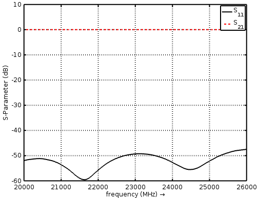
Plot the s-parameters:
figure
plot(freq*1e-6,20*log10(abs(s11)),'k-','Linewidth',2);
xlim([freq(1) freq(end)]*1e-6);
grid on;
hold on;
plot(freq*1e-6,20*log10(abs(s21)),'r--','Linewidth',2);
l = legend('S_{11}','S_{21}','Location','Best');
set(l,'FontSize',12);
ylabel('S-Parameter (dB)','FontSize',12);
xlabel('frequency (MHz) \rightarrow','FontSize',12);
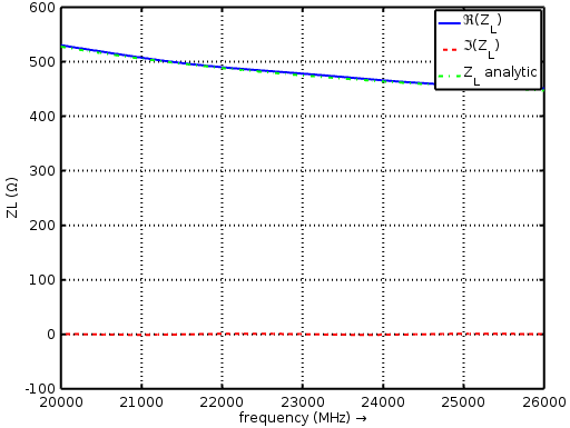
Compare analytic and numerical wave-impedance:
figure
plot(freq*1e-6,real(ZL),'Linewidth',2);
hold on;
grid on;
plot(freq*1e-6,imag(ZL),'r--','Linewidth',2);
plot(freq*1e-6,ZL_a,'g-.','Linewidth',2);
ylabel('ZL (\Omega)','FontSize',12);
xlabel('frequency (MHz) \rightarrow','FontSize',12);
xlim([freq(1) freq(end)]*1e-6);
l = legend('\Re(Z_L)','\Im(Z_L)','Z_L analytic','Location','Best');
set(l,'FontSize',12);
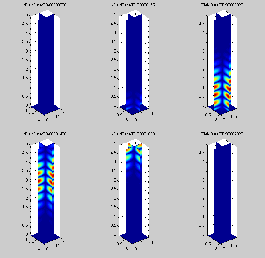
Plot the field dumps:
figure
dump_file = [Sim_Path '/Et.h5'];
PlotArgs.slice = {a/2*unit b/2*unit 0};
PlotArgs.pauseTime=0.01;
PlotArgs.component=0;
PlotArgs.Limit = 'auto';
PlotHDF5FieldData(dump_file, PlotArgs)


