Visualization of Results

From openEMS

The simulation results can be viewed and analyzed in many ways using Matlab/Octave functions. Here are some examples.

Time Domain

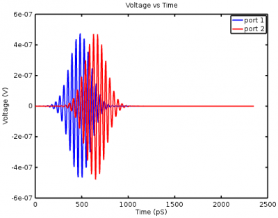
Here is an example of the voltage waveforms in the rectangular waveguide tutorial which has a section of waveguide with ports at each end. After the simulation is complete, the plot frequency range is defined and calcPort is run.

f_start = 20e9;
f_0     = 24e9;
f_stop  = 26e9;
% ...
freq = linspace(f_start,f_stop,201);
port = calcPort(port, Sim_Path, freq);

The time values and the total voltage values are extracted from the data structures for the ports and plotted. The blue curve is the active port and the red curve shows the wave incident on the second port.

figure
plot( 1e12*port{1}.ut.time, port{1}.ut.tot, 'b-', 'Linewidth', 2 );
hold on
plot( 1e12*port{1}.ut.time, port{2}.ut.tot, 'r-', 'Linewidth', 2 );
title( 'Voltage vs Time' );
xlabel( 'Time (pS)' );
ylabel( 'Voltage (V)' );
legend( 'port 1','port 2');

Time-Domain plot

Frequency Domain

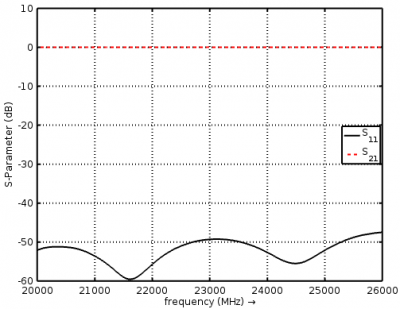
Frequently in microwave engineering we want to view the s-parameters, just as we would with a vector network analyzer. Here is an example taken from the rectangular waveguide tutorial. After the simulation is complete, the plot frequency range is defined and calcPort is run. (Note that it should only be necessary to run calcPort once, and then numerous plots can be made from the port data structure.)

f_start = 20e9;
f_0     = 24e9;
f_stop  = 26e9;
% ...
freq = linspace(f_start,f_stop,201);
port = calcPort(port, Sim_Path, freq);

Next, components of the port structure can be used in calculations and the results plotted. Here is the calculation of s11 and s21 using incident and reflected frequency-domain voltages:

s11 = port{1}.uf.ref./ port{1}.uf.inc;
s21 = port{2}.uf.ref./ port{1}.uf.inc;

And the curves plotted in dB:

figure
plot(freq*1e-6,20*log10(abs(s11)),'k-','Linewidth',2);
xlim([freq(1) freq(end)]*1e-6);
grid on;
hold on;
plot(freq*1e-6,20*log10(abs(s21)),'r--','Linewidth',2);
l = legend('S_{11}','S_{21}','Location','East');
set(l,'FontSize',12);
ylabel('S-Parameter (dB)','FontSize',12);
xlabel('frequency (MHz) \rightarrow','FontSize',12);

S-Parameter plot

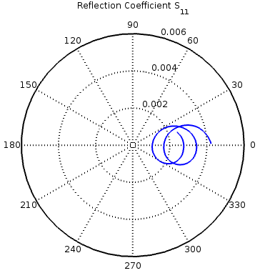
The reflection coefficient can also be plotted on a polar plot (Smith Chart). Note that in this example that the radius of the outer circle is much less than 1 because the waveguide is well matched and auto-scaling zooms into the centre of the plot.

polar(arg(s11), abs(s11));
title( 'Reflection Coefficient S_{11}' );

Smith Chart plot

Radiation Patterns

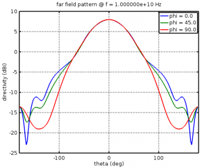
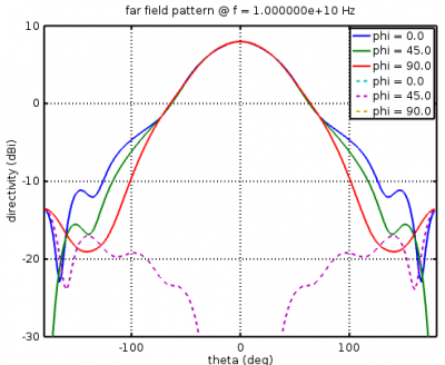
For antennas, radiation patterns are an important property to plot. Assuming that the NF2FF box has been set up in the simulation, after the simulation the CalcNF2FF function transforms the near-field data at frequency f0 to far-field cuts over the range thetaRange on cuts phiCuts (in this case 0, 45, and 90 degrees).

thetaRange = (0:2:359) - 180;
phiCuts = [0 45 90];
nf2ff = CalcNF2FF(nf2ff, Sim_Path, f0, thetaRange*pi/180, phiCuts*pi/180);

The openEMS function plotFFdB plots the radiation patterns.

figure
plotFFdB(nf2ff,'xaxis','theta','param',[1 2 3]);
axis([-180 180]);

Radiation pattern plot

However, plotFFdB plots |E| which has the co- and cross-polarized components of the electric field combined, and antenna engineers often plot the two polarization responses as separate curves. Part of the structure returned by CalcNF2FF are orthogonal field components aligned in the phi direction and the theta direction. These components can be extracted with:

E_theta = nf2ff.E_theta{freq_index} / max(nf2ff.E_norm{freq_index}(:));
E_phi = nf2ff.E_phi{freq_index} / max(nf2ff.E_norm{freq_index}(:));

Conversion to co and cross is straightforward:

% Convert from E_theta and E_phi to co- and cross-pol as per
% Ludwig's third definition.
% Ref.: Milligan, Modern Antenna Design, 2005, p.22
% [ E_co] = [cos(phi)  -sin(phi)] [E_phi  ]
% [ E_cx] = [sin(phi)   cos(phi)] [E_theta]
 
E_co = E_theta.*cos(nf2ff.phi) - E_phi.*sin(nf2ff.phi);
E_cx = E_theta.*sin(nf2ff.phi) + E_phi.*cos(nf2ff.phi);
 
E_co_log = 20*log10(E_co) + 10*log10(nf2ff.Dmax(freq_index));
E_cx_log = 20*log10(E_cx) + 10*log10(nf2ff.Dmax(freq_index));

These can be plotted on a single graph with solid lines representing the co-polarized patterns and dashed lines the cross-polarized patterns.

xax = nf2ff.theta;
yax1 = E_co_log(:,param);
yax2 = E_cx_log(:,param);
h = plot( xax/pi*180, yax1, xax/pi*180, yax2, '--' );

(In this example param = [1 2 3] to specify the three phi-cuts.)

Radiation pattern plot with co- and cross-polarized responses.

A modified version of plotFFdB plots the co- and cross-polarized patterns: File:PlotFFcocx.m.